Fitting stellar parameters
The central purpose of isochrones is to infer the physical properties of stars given arbitrary observations. This is accomplished via the StarModel object. For simplest usage, a StarModel is initialized with a ModelGridInterpolator and observed properties, provided as (value, uncertainty) pairs. Also, while the vanilla StarModel object (which is mostly the same as the isochrones v1 StarModel object) can still be used to fit a single star, isochrones v2 has a
new SingleStarModel available, that has a more optimized likelihood implementation, for significantly faster inference.
Defining a star model
First, let’s generate some “observed” properties according to the model grids themselves. Remember that .generate() only works with the evolution track interpolator.
[1]:
from isochrones.mist import MIST_EvolutionTrack, MIST_Isochrone

track = MIST_EvolutionTrack()

mass, age, feh, distance, AV = 1.0, 9.74, -0.05, 100, 0.02

# Using return_dict here rather than return_df, because we just want scalar values
true_props = track.generate(mass, age, feh, distance=distance, AV=AV, return_dict=True)
true_props
[1]:
{'nu_max': 2617.5691700617886,
 'logg': 4.370219109480715,
 'eep': 380.0,
 'initial_mass': 1.0,
 'radius': 1.0813017873811603,
 'logTeff': 3.773295968705084,
 'mass': 0.9997797219140423,
 'density': 1.115827651504971,
 'Mbol': 4.4508474939623826,
 'phase': 0.0,
 'feh': -0.09685557997282962,
 'Teff': 5934.703385987951,
 'logL': 0.11566100241504726,
 'delta_nu': 126.60871562200438,
 'interpolated': 0.0,
 'star_age': 5522019067.711771,
 'age': 9.74119762492735,
 'dt_deep': 0.0036991465241712263,
 'J': 8.435233804866742,
 'H': 8.124109062114325,
 'K': 8.09085566863133,
 'G': 9.387465543790636,
 'BP': 9.680097761608252,
 'RP': 8.928888526297722,
 'W1': 8.079124865544092,
 'W2': 8.090757185192754,
 'W3': 8.06683507215844,
 'TESS': 8.923262483762786,
 'Kepler': 9.301490687837552}
Now, we can define a starmodel with these “observations”, this time using the isochrone grid interpolator. We use the optimized SingleStarModel object.
[2]:
from isochrones import SingleStarModel, get_ichrone

mist = get_ichrone('mist')

uncs = dict(Teff=80, logg=0.1, feh=0.1, phot=0.02)
props = {p: (true_props[p], uncs[p]) for p in ['Teff', 'logg', 'feh']}
props.update({b: (true_props[b], uncs['phot']) for b in 'JHK'})

# Let's also give an appropriate parallax, in mas
props.update({'parallax': (1000./distance, 0.1)})

mod = SingleStarModel(mist, name='demo', **props)
And we can see the prior, likelihood, and posterior at the true parameters:
[3]:
eep = mist.get_eep(mass, age, feh, accurate=True)
pars = [eep, age, feh, distance, AV]

mod.lnprior(pars), mod.lnlike(pars), mod.lnpost(pars)
[3]:
(-23.05503287088296, -20.716150242083508, -43.77118311296647)
If we stray from these parameters, we can see the likelihood decrease:
[4]:
pars2 = [eep + 3, age - 0.05, feh + 0.02, distance, AV]
mod.lnprior(pars2), mod.lnlike(pars2), mod.lnpost(pars2)
[4]:
(-23.251706955307853, -85.08590699022739, -108.33761394553524)
How long does a posterior evaluation take?
[5]:
%timeit mod.lnpost(pars)
1000 loops, best of 3: 369 µs per loop
[6]:
from isochrones import BinaryStarModel

mod2 = BinaryStarModel(mist, **props)
[7]:
pars2 = [eep, eep - 20, age, feh, distance, AV]
%timeit mod2.lnpost(pars2)
The slowest run took 373.39 times longer than the fastest. This could mean that an intermediate result is being cached.
1000 loops, best of 3: 429 µs per loop
[8]:
from isochrones import TripleStarModel
mod3 = TripleStarModel(mist, **props)
pars3 = [eep, eep-20, eep-40, age, feh, distance, AV]
%timeit mod3.lnpost(pars3)
1000 loops, best of 3: 541 µs per loop
Priors
As you may have noticed, we have not explictly defined any priors on our parameters. They were defined for you, but you may wish to know what they are, and/or to change them.
[9]:
mod._priors
[9]:
{'mass': <isochrones.priors.ChabrierPrior at 0x1c47e270f0>,
 'feh': <isochrones.priors.FehPrior at 0x1c47e27358>,
 'age': <isochrones.priors.AgePrior at 0x1c47e27748>,
 'distance': <isochrones.priors.DistancePrior at 0x1c47e27390>,
 'AV': <isochrones.priors.AVPrior at 0x1c47e27400>,
 'eep': <isochrones.priors.EEP_prior at 0x1c47e274e0>}
You can sample from these priors:
[10]:
samples = mod.sample_from_prior(1000)
samples
[10]:
| age | feh | distance | AV | eep | |
|---|---|---|---|---|---|
| 0 | 9.775384 | 0.004928 | 9585.312354 | 0.058294 | 415 |
| 1 | 9.690678 | 0.318313 | 5460.742158 | 0.212007 | 295 |
| 2 | 9.317426 | -0.008935 | 5381.226921 | 0.144259 | 265 |
| 3 | 9.721345 | -0.131058 | 7867.502875 | 0.228851 | 295 |
| 4 | 9.374286 | -0.325079 | 9590.728624 | 0.954659 | 350 |
| 5 | 9.293293 | 0.229220 | 9574.055273 | 0.713866 | 293 |
| 6 | 9.941975 | 0.178338 | 7788.336554 | 0.100102 | 272 |
| 7 | 9.436477 | 0.231631 | 9148.585364 | 0.204715 | 314 |
| 8 | 9.743647 | -0.396267 | 6767.456426 | 0.383272 | 460 |
| 9 | 9.607588 | -0.236938 | 4317.243131 | 0.795216 | 327 |
| 10 | 10.057273 | -0.236801 | 9031.515061 | 0.488995 | 314 |
| 11 | 9.645887 | -0.338786 | 9055.303060 | 0.408045 | 1702 |
| 12 | 9.997611 | -0.214726 | 8452.833760 | 0.398581 | 327 |
| 13 | 9.926111 | -0.063765 | 9726.761618 | 0.544188 | 321 |
| 14 | 9.845896 | -0.106017 | 9148.167681 | 0.455272 | 292 |
| 15 | 9.761015 | -0.051480 | 8247.211954 | 0.379722 | 253 |
| 16 | 9.286601 | -0.186755 | 7113.433648 | 0.504276 | 451 |
| 17 | 8.124025 | -0.138695 | 9335.360257 | 0.445926 | 380 |
| 18 | 9.357514 | 0.067101 | 7737.470105 | 0.752912 | 300 |
| 19 | 9.595645 | 0.107345 | 7115.589991 | 0.231624 | 420 |
| 20 | 9.933118 | -0.048234 | 8424.490753 | 0.139511 | 1692 |
| 21 | 10.105196 | 0.292670 | 9485.836532 | 0.366055 | 331 |
| 22 | 10.040531 | 0.014999 | 9296.367644 | 0.185203 | 314 |
| 23 | 9.967137 | 0.000672 | 8552.101985 | 0.791577 | 254 |
| 24 | 10.128790 | -0.176654 | 6727.495813 | 0.494750 | 345 |
| 25 | 9.854273 | -0.183929 | 5380.753272 | 0.945978 | 407 |
| 26 | 9.808855 | 0.074433 | 8664.219066 | 0.692098 | 455 |
| 27 | 9.917164 | 0.202846 | 7496.956324 | 0.363808 | 389 |
| 28 | 9.630302 | -0.373880 | 8555.632299 | 0.287120 | 322 |
| 29 | 9.179908 | -0.199734 | 9856.026771 | 0.303459 | 300 |
| ... | ... | ... | ... | ... | ... |
| 970 | 10.086391 | 0.106938 | 7592.165249 | 0.180709 | 314 |
| 971 | 10.085083 | -0.036016 | 7027.634747 | 0.314156 | 299 |
| 972 | 9.287464 | 0.265288 | 6042.848103 | 0.144724 | 402 |
| 973 | 9.955503 | -0.080510 | 6262.492050 | 0.611200 | 327 |
| 974 | 9.616142 | -0.342509 | 5069.839242 | 0.567513 | 349 |
| 975 | 10.075706 | -0.130103 | 5829.432844 | 0.892020 | 299 |
| 976 | 10.028535 | 0.193184 | 4257.798238 | 0.293645 | 329 |
| 977 | 9.574676 | 0.085395 | 9752.502653 | 0.703944 | 357 |
| 978 | 9.556853 | -0.140753 | 8530.526505 | 0.871235 | 334 |
| 979 | 9.821810 | -0.118098 | 8972.965633 | 0.026728 | 397 |
| 980 | 10.105103 | 0.104010 | 9992.769437 | 0.343932 | 292 |
| 981 | 9.853596 | -0.118408 | 6035.299187 | 0.686813 | 254 |
| 982 | 9.312975 | -0.038113 | 8689.991781 | 0.047170 | 324 |
| 983 | 8.971418 | 0.238024 | 5797.572151 | 0.773175 | 268 |
| 984 | 9.664546 | -0.028603 | 9719.254429 | 0.707218 | 347 |
| 985 | 9.924745 | -0.216946 | 9422.814918 | 0.292175 | 292 |
| 986 | 9.624291 | -0.034933 | 4359.825182 | 0.661057 | 317 |
| 987 | 9.947794 | -0.264508 | 8355.572420 | 0.301372 | 292 |
| 988 | 9.766796 | 0.070148 | 9155.900363 | 0.597846 | 292 |
| 989 | 9.960194 | 0.026427 | 7655.336536 | 0.002166 | 265 |
| 990 | 9.488527 | -0.094431 | 9896.426901 | 0.662185 | 271 |
| 991 | 10.105075 | 0.145627 | 3359.853867 | 0.416843 | 489 |
| 992 | 9.994699 | -0.246844 | 6033.657596 | 0.198885 | 271 |
| 993 | 9.369871 | 0.052412 | 2669.191340 | 0.294969 | 317 |
| 994 | 9.903893 | 0.176871 | 8832.480953 | 0.128152 | 295 |
| 995 | 9.864971 | 0.142656 | 9366.389176 | 0.782361 | 347 |
| 996 | 9.968736 | 0.027372 | 8748.808096 | 0.300267 | 351 |
| 997 | 9.525780 | 0.005426 | 6651.084393 | 0.508013 | 247 |
| 998 | 9.290521 | -0.064370 | 8489.972371 | 0.615413 | 296 |
| 999 | 10.131466 | 0.077783 | 8694.197822 | 0.833533 | 271 |
1000 rows × 5 columns
Remember, these are the fit parameters:
[11]:
mod.param_names
[11]:
('eep', 'age', 'feh', 'distance', 'AV')
Let’s turn this into a dataframe, and visualize it.
[12]:
import pandas as pd
import holoviews as hv
import hvplot.pandas
hv.extension('bokeh')

def plot_samples(samples):
    df = pd.DataFrame(samples, columns=['eep', 'age', 'feh', 'distance', 'AV'])
    df['mass'] = mod.ic.interp_value([df.eep, df.age, df.feh], ['mass'])
    return hv.Layout([df.hvplot.hist(c).options(width=300) for c in df.columns]).cols(3)

plot_samples(samples)


[12]:
Note that there are some built-in defaults here to be aware of. The metallicity distribution is based on a local metallicity prior from SDSS, the distance prior has a maximum distance of 10kpc, and AV is flat from 0 to 1. Now, let’s change our distance prior to only go out to 1000pc, and our metallicity distribution to be flat between -2 and 0.5.
[13]:
from isochrones.priors import FlatPrior, DistancePrior
mod.set_prior(feh=FlatPrior((-2, 0.5)), distance=DistancePrior(1000))
[14]:
plot_samples(mod.sample_from_prior(1000))
[14]:
Also note that the default mass prior is the Chabrier broken powerlaw, which is nifty:
[15]:
pd.Series(mod._priors['mass'].sample(10000), name='mass').hvplot.hist(bins=100, bin_range=(0, 5))
[15]:
You can also define a metallicity prior to have a different mix of halo and (local) disk:
[16]:
from isochrones.priors import FehPrior

pd.Series(FehPrior(halo_fraction=0.5).sample(10000), name='feh').hvplot.hist()
[16]:
Sampling the posterior
Once you have defined your stellar model and are happy with your priors, you may either execute your optimization/sampling method of choice using the .lnpost() method as your posterior, or you may use the built-in MultiNest fitting routine with .fit(). One thing to note especially is that the MultiNest chains get automatically created in a chains subdirectory from wherever you execute .fit(), with a basename for the files that you can access with:
[17]:
mod.mnest_basename
[17]:
'./chains/demo-mist-single-'
This can be changed or overwritten in two ways, which is often a good idea to avoid clashes between different fits with the same default basename. You can either by pass an explicit basename keyword to .fit(), or you can set a name attribute, as we did when initializing this model. OK, now we will run the fit. This will typically take a few minutes (unless the chains for the fit have already completed, in which case it will be read in and finish quickly).
[18]:
mod.fit()
INFO:root:MultiNest basename: ./chains/demo-mist-single-
The posterior samples of the sampling parameters are available in the .samples attribute. Note that this is different from the original vanilla StarModel object (the one fully backward-compatible with isochrones v1), which contained both sampling parameters and derived parameters at the values of those samples.
[19]:
mod.samples.head()
[19]:
| eep | age | feh | distance | AV | lnprob | |
|---|---|---|---|---|---|---|
| 0 | 306.566211 | 8.867352 | -0.084787 | 99.754595 | 0.128567 | -51.124447 |
| 1 | 385.106002 | 9.744207 | 0.179155 | 99.818131 | 0.492972 | -49.729296 |
| 2 | 301.018106 | 8.745846 | -0.030370 | 100.473273 | 0.579248 | -49.425361 |
| 3 | 259.680008 | 8.214644 | 0.010053 | 98.376332 | 0.363801 | -48.479515 |
| 4 | 380.210824 | 9.700131 | -0.178482 | 99.398149 | 0.633511 | -48.453800 |
[20]:
mod.samples.describe()
[20]:
| eep | age | feh | distance | AV | lnprob | |
|---|---|---|---|---|---|---|
| count | 5344.000000 | 5344.000000 | 5344.000000 | 5344.000000 | 5344.000000 | 5344.000000 |
| mean | 373.193478 | 9.686096 | -0.045856 | 100.021338 | 0.146828 | -40.820994 |
| std | 19.800711 | 0.181541 | 0.076720 | 0.993574 | 0.111217 | 1.525383 |
| min | 217.053516 | 7.653568 | -0.301781 | 96.356886 | 0.000078 | -51.124447 |
| 25% | 359.164345 | 9.599845 | -0.098619 | 99.355457 | 0.060500 | -41.532015 |
| 50% | 375.054046 | 9.712589 | -0.045498 | 100.013786 | 0.124330 | -40.468810 |
| 75% | 387.980876 | 9.806347 | 0.007986 | 100.685282 | 0.208648 | -39.723250 |
| max | 420.506604 | 10.089448 | 0.193737 | 103.660815 | 0.755101 | -38.472525 |
The derived parameters are available in .derived_samples (StarModel on its own does not have this attribute):
[21]:
mod.derived_samples.head()
[21]:
| eep | age | feh | mass | initial_mass | radius | density | logTeff | Teff | logg | ... | BP_mag | RP_mag | W1_mag | W2_mag | W3_mag | TESS_mag | Kepler_mag | parallax | distance | AV | |
|---|---|---|---|---|---|---|---|---|---|---|---|---|---|---|---|---|---|---|---|---|---|
| 0 | 306.566211 | 8.867352 | -0.068345 | 1.098369 | 1.098407 | 1.037567 | 1.391965 | 3.790660 | 6176.198702 | 4.447143 | ... | 9.673531 | 8.942160 | 8.124458 | 8.127637 | 8.109427 | 8.936103 | 9.307189 | 10.024601 | 99.754595 | 0.128567 |
| 1 | 385.106002 | 9.744207 | 0.159727 | 1.057168 | 1.057394 | 1.141433 | 1.002494 | 3.763116 | 5796.649384 | 4.347338 | ... | 10.181673 | 9.176220 | 8.004902 | 8.018791 | 7.972552 | 9.164784 | 9.669073 | 10.018220 | 99.818131 | 0.492972 |
| 2 | 301.018106 | 8.745846 | -0.011900 | 1.152686 | 1.152721 | 1.096043 | 1.237448 | 3.796728 | 6262.723700 | 4.420403 | ... | 9.982068 | 9.077651 | 8.030137 | 8.021413 | 7.994322 | 9.066848 | 9.529013 | 9.952896 | 100.473273 | 0.579248 |
| 3 | 259.680008 | 8.214644 | 0.048588 | 1.147012 | 1.147023 | 1.065911 | 1.338449 | 3.790769 | 6177.197873 | 4.442458 | ... | 9.830745 | 8.993534 | 8.044905 | 8.045347 | 8.020660 | 8.985118 | 9.409833 | 10.165047 | 98.376332 | 0.363801 |
| 4 | 380.210824 | 9.700131 | -0.257214 | 1.010634 | 1.010881 | 1.123263 | 1.005285 | 3.787708 | 6134.335252 | 4.341725 | ... | 10.085126 | 9.130129 | 7.986850 | 7.974103 | 7.941984 | 9.117792 | 9.608276 | 10.060550 | 99.398149 | 0.633511 |
5 rows × 30 columns
You can make a corner plot of the fit parameters as follows:
[22]:
%matplotlib inline

mod.corner_params();  # Note, this is also new in v2.0, for the SingleStarModel object
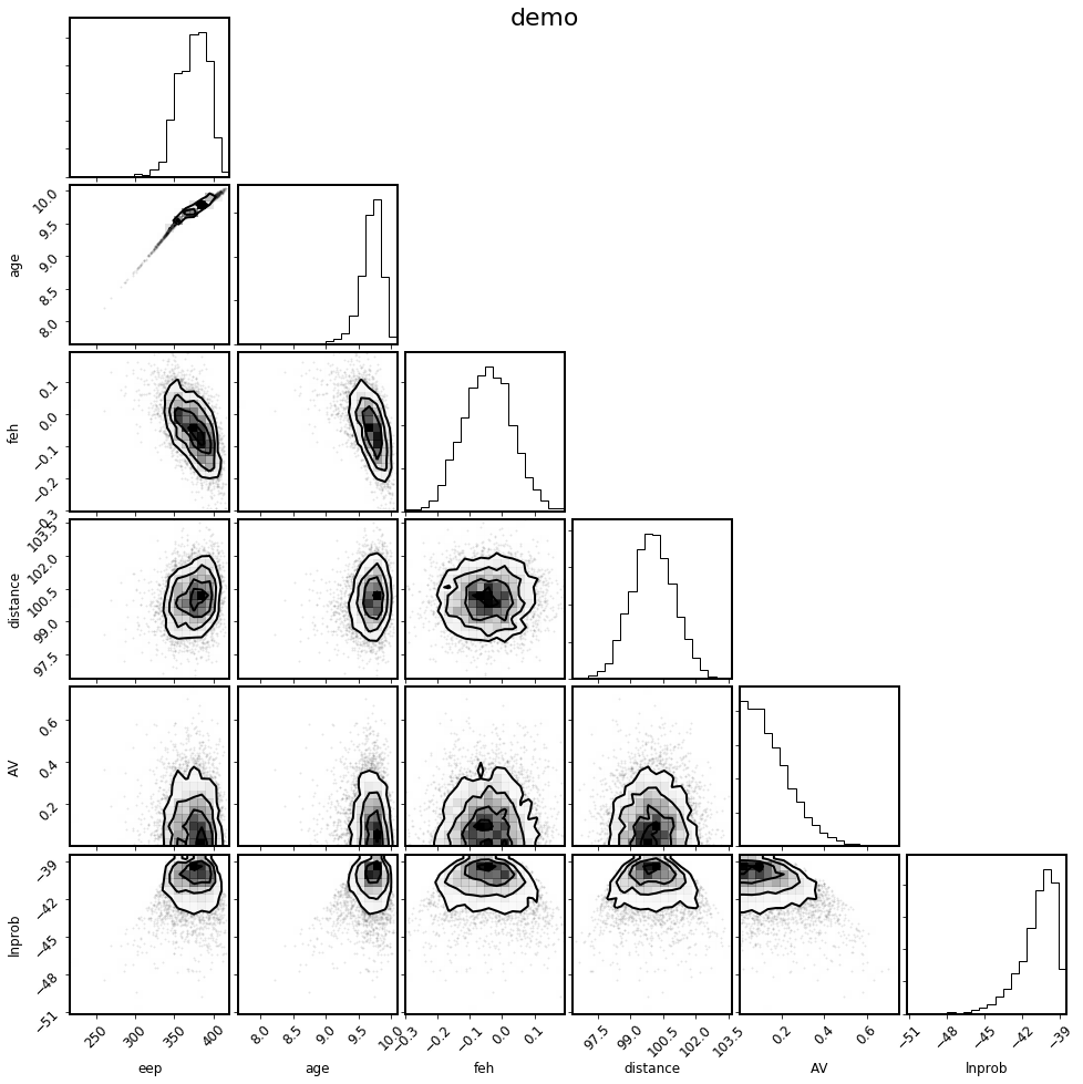
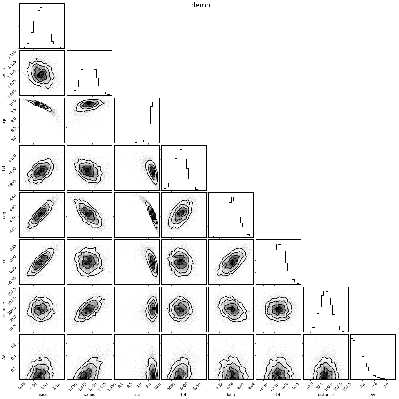
There is also a convenience method to select the parameters of physical interest.
[23]:
mod.corner_physical();
It can also be instructive to see how the derived samples of the observed parameters compare to the observations themselves; the shortcut to this is with the .corner_observed() convenience method:
[24]:
mod.corner_observed();
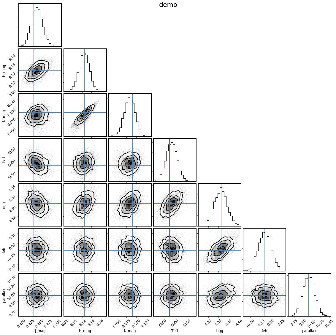
This looks good, because we generated the synthetic observations directly from the same stellar model grids that we used to fit. For real data, this is an important figure to look at to see if any of the observations appear to be inconsistent with the others, and to see if the model is a good fit to the observations.
Generically, you can also make a corner plot of arbitrary derived parameters as follows:
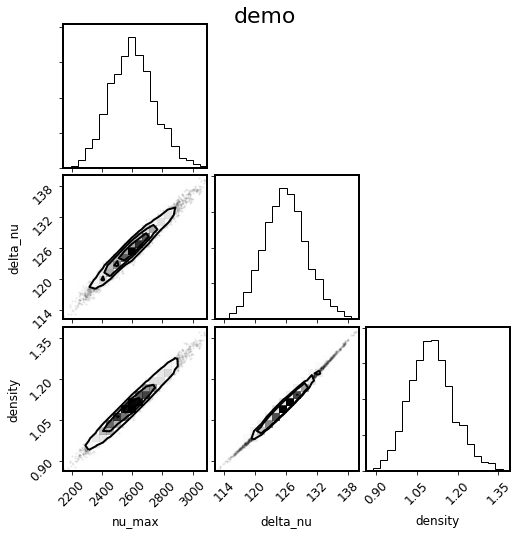
[25]:
mod.corner_derived(['nu_max', 'delta_nu', 'density']);